
Market policy equilibrium embedded in probabilistic world models
Embedding policy games inside a probabilistic world model, from the Fed to sanctions and tariffs.
- By
- PolyBridge Research
- Topic
- Policy–market equilibrium
- Date
- Reading time
- 9 min
A loop between policy and prices
Policymakers set levers that markets price, and they watch that pricing when they decide. A central bank rarely delivers a decision the market has not priced. A government that announces a tariff watches the reaction in equities and bonds. An oil producer sets output with one eye on the futures curve.
The market, in turn, prices what it expects the policymaker to do. Each side responds to the other. That makes the relationship a game: the policymaker's choice depends on the market's pricing, and the pricing depends on the expected choice.
Most forecasting models treat one side as fixed. A reaction-function model of a central bank ignores the market. A model that reads market-implied probabilities takes them as given.
At PolyBridge we build probabilistic world models: causal graphs over economic concepts, written as probabilistic programs and fitted to historical data and forward-dated market evidence such as futures and prediction markets. This post sets out how a policy–market game can sit inside a world model's data-generating process, what that reveals, where the inference is hard, and how the same structure extends from the Fed to geoeconomic levers such as sanctions, price caps and tariffs.
In brief
- Policymakers and markets watch each other. Treating that as a game shows what each side wants, not only what it did.
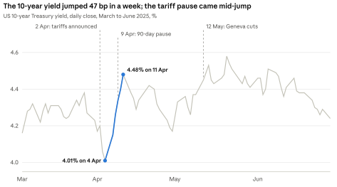
- It measures how far a policymaker follows markets. In April 2025 a 47 bp jump in bond yields came days before a tariff pause; this approach puts a number on that kind of pain threshold.
- It ranks policy levers (tariffs, sanctions, price caps) by effect per unit of cost at home, after other countries respond.
- It shows which market prices are cheap to push and should be trusted less.
The technical sections follow. Readers after the takeaways can skip to Case 3 and "What the game reveals".
How the game works
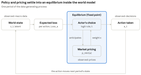
An actor (a central bank, a government, an oil producer) chooses an action a from a small set: cut, hold or hike; raise or lower a tariff; tighten or loosen a cap. The world model computes Loss_a: how far each action would leave the actor from its goals, where lower is better. Markets supply p_mkt(a): the probability market prices put on each action, for example the chance of a rate cut implied by fed funds futures.
Loss_a is an expected loss. z_t is the current state of the economy (inflation, unemployment, oil supply and so on), z' is next period's state, and θ stands for the world model's fitted parameters. ℓ scores how bad an outcome is for the actor. do(a) means the action is set to a by hand, so the model shows what the action causes rather than the conditions in which it is usually taken. The expectation averages ℓ over the possible next-period states:
An action whose outcome is uncertain carries a higher expected loss than one with the same central outcome and less spread.
The actor picks actions with a logit (quantal response) rule (McKelvey and Palfrey, 1995): lower-loss actions are more likely, and actions the market has priced get extra weight.
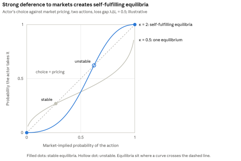
Two parameters carry the behaviour. λ (consistency) measures how reliably the actor picks the lowest-loss action: at λ = 0 it picks at random, and as λ grows it almost always picks the best action. κ (deference to markets) measures how much weight the actor gives to what markets expect: at κ = 0 it ignores pricing and follows its own goals alone, which is a standard reaction function; at larger κ, an action the market has priced becomes more likely to be chosen.
The market prices what it expects the actor to do, so in equilibrium pricing and behaviour agree. The equilibrium is a fixed point. p*(a) is the equilibrium pricing: the probabilities that, once the actor reacts to them, reproduce themselves:
For κ < 1 the fixed point is unique and damped iteration converges. For κ ≥ 1 self-fulfilling equilibria appear: if the market prices an action strongly enough, the actor takes it whatever its loss.
Observed pricing is treated as a noisy view of the equilibrium, and observed decisions as draws from the actor's choice given the pricing it actually faced:
c sets how closely observed pricing tracks the equilibrium: the larger c, the less noise. Each period, the full generative sequence is:
- State: z_t ~ p(z_t | z_{t−1}, a_{t−1}, θ), so last period's action drives the state.
- Expected losses Loss_a(z_t, θ), then the equilibrium p*_t.
- Pricing: p_mkt,t ~ Dirichlet(c p*_t).
- Decision: a_t ~ Categorical(P_actor(p_mkt,t)).
- Macro data: y_t ~ p(y_t | z_t). y_t are the published statistics (CPI, payrolls, oil output) that measure the state with noise.
The game sits inside the generative model; inference runs around it. Because actions feed the next state, prices and decisions inform the world model's state and parameters jointly with the macro data. Inference returns a posterior over the actor's preferences (the weights inside Loss), λ and κ, alongside the rest of the model. This is 'inverse game theory': inferring what an actor wants from what it does and from what markets expect it to do.
Case 1: the Fed and the market
The Federal Reserve is a clear example. It meets about eight times a year, its decisions are public, and fed funds futures have priced each decision for decades (Kuttner, 2001).
The Fed chooses a rate change Δr from {−0.25, 0, +0.25} (the code below shows this case; larger moves such as 50 and 75bp extend the set). Each action moves next-period gaps in core inflation (π = core inflation − 2%) and unemployment (u = unemployment − u*, where u* is the unemployment rate consistent with stable inflation):
π'_a and u'_a are the gaps next period if the Fed takes action a. b_π and b_u are how far a rate change moves each gap within a period. L_a is the Fed's loss: the squared gaps, so misses in either direction count. α is the weight on inflation against unemployment: at α = 0.5 they count equally, and α near 1 means the Fed cares mostly about inflation. Plugged into the choice rule and fitted to decisions and pricing, the model returns α, λ and κ, and forecasts each decision.
A natural check is whether adding market pricing (κ > 0) predicts the Fed's decisions better than a reaction function alone (κ = 0). It would, for a reason worth unpacking.
Who leads whom? A week before a meeting, markets already have some idea what the Fed will do. Speeches, minutes and the occasional press report steer pricing in advance, and the Fed has rarely surprised markets in recent decades. Pricing predicts decisions whether the Fed follows the market or the market follows the Fed. κ also absorbs everything the simple loss misses. A large κ fitted naively says "pricing contains information", not "the Fed defers to markets".
Three approaches help:
- Earlier pricing. Use pricing from four to six weeks before a meeting, before the pre-meeting quiet period and most guidance.
- Variation the Fed did not cause. Use data surprises that land after pricing has settled, and episodes where pricing moved sharply for outside reasons, such as the shift to a 75bp hike in June 2022, priced in the days before the meeting after a press report.
- Communication as a separate input. Add Fed speech and minutes signals to the loss side, so κ is not credited with them. Statements move markets separately from actions (Gürkaynak, Sack and Swanson, 2005).
With these, κ becomes an estimate of deference rather than a measure of how informed the market is.
Why it is worth measuring. Rate forecasts drive bond portfolios, pension liabilities and stress scenarios. Whether the Fed leads or follows markets is a long-running question about its independence, and κ tracked over time puts a number on it. This is deference to market pricing, which is separate from deference to the government. It is also separate from the "Fed put": the finding that stock market falls predict Fed easing, through their effect on the Fed's growth outlook (Cieslak and Vissing-Jorgensen, 2021). If κ > 0, pricing is also a lever on policy: whoever moves pricing gains some influence. Fed funds futures are deep enough that this lever is very expensive to pull.
Case 2: geoeconomic levers
The Fed game is the domestic case of a general pattern. States set economic levers (tariffs, sanctions, export controls, oil output, currency fixing), markets price those levers, and states respond to the pricing. Geoeconomics adds three things.
| Domestic (Fed) | Geoeconomic | |
|---|---|---|
| Actor | Central bank | A state: trade or sanctions authority, oil producer, central bank managing a currency |
| Lever | Interest rates | Tariffs, sanctions, export controls, output, currency fixing |
| Market pricing the lever | Fed funds futures, Fed event contracts | Tariff and sanctions event contracts, Brent futures, offshore currency markets |
| Other players | None | The target state responds; third countries and firms reroute |
| Costs | Domestic only | Split between target and home |
| Can pricing be pushed? | Too deep to push cheaply | Often thin, so cheap to push |
The choice rule and the fixed point are unchanged. What changes is that several players solve the game together, the cost of a lever lands partly at home, and thin geopolitical markets can be moved by someone with a stake in the outcome.
Worked example: the Russian oil price cap. In December 2022 the G7 capped the price at which Western services could support Russian crude exports at US$60 per barrel; the EU and UK later lowered their caps. The Urals discount to Brent widened, then narrowed as a shadow fleet grew to carry oil outside the cap. The question is which lever cuts Russian oil revenue most for the least cost to fuel prices at home, once the other players respond.
| Player | Actions | Payoff |
|---|---|---|
| US and G7 (move first) | Cap level; enforcement low / high; strategic reserve release none / some | w1·(cut in Russian oil revenue) − w2·(rise in home fuel prices) |
| Russia | Sell within the cap / ship via shadow fleet / cut output | Oil revenue − shipping and evasion costs |
| Saudi Arabia (OPEC+) | Cut / hold / raise output | Revenue + v·market share |
| US shale | Drilling low / high | Profit at the expected price |
Rev_RU is Russia's oil revenue, Q_RU its export volume and P_Brent the Brent price. D is the discount at which Russian crude sells: d_0 is the base discount, d_1 how much tighter enforcement widens it, and d_2 how much shadow-fleet capacity narrows it. Q_SA and Q_shale are Saudi and US shale output. In the table, w1 and w2 are the G7's weights on cutting Russian revenue and on keeping fuel prices down at home, and v is Saudi Arabia's weight on market share relative to revenue.
The Urals discount, tanker-tracked export volumes, Brent futures, OPEC+ decisions, rig counts and US fuel prices are all observed, and supply shocks such as a Strait of Hormuz disruption come from a model of oil supply. The fitted game ranks levers by revenue cut per unit of home cost, recovers Saudi Arabia's trade-off between revenue and market share, and lets us change the rules (a lower cap, tighter enforcement, reserve support) and re-solve. It also reproduces the evasion response: a cap that bites on what it can measure invites routing around it.
The same structure covers OPEC+ output decisions against Brent futures, the People's Bank of China's daily yuan fix against offshore pricing, and Japanese currency intervention against yen option markets. Shipping disruption in the Taiwan Strait would enter as a supply shock, as Hormuz does for oil. US–China trade is the subject of Case 3.
Case 3: tariffs and the bond market
US–China trade in 2025 is a clear recent case of a policy decision turning on market pricing.
- On 2 April 2025 the US announced broad "reciprocal" tariffs. Equities fell sharply. Treasury yields fell for two days, then rose instead of falling further: the 10-year went from 4.01% on 4 April to 4.48% on 11 April, the reverse of the usual flight to safety.
- On 9 April the US paused most of the new tariffs for 90 days while raising tariffs on China. The president said the bond market had been getting "yippy" (Fortune).
- In May, after talks in Geneva, both sides cut tariffs by 115 percentage points for 90 days (Gibson Dunn). In October China expanded export controls on rare earths and the US threatened an extra 100% tariff (S&P Global). At a meeting in Busan on 30 October both stepped back: China suspended the new controls for a year and the US cut some tariffs (Reuters via gCaptain).
Two kinds of market influence. The episode separates two ways pricing can enter a decision.
- Market as forecast. The actor defers to what the market expects it to do. This is κ in the choice rule.
- Market as cost. The market's reaction is itself part of the loss. A tariff that pushes up borrowing costs is costly whatever the market expected.
The tariff pause looks like the second. The US loss for each action then includes expected market moves under that action, taken from the world model:
w1 to w4 are the administration's weights on leverage over trading partners, on the rise in the 10-year Treasury yield (Δy_10), on the fall in equities and on inflation. The fitted w2 gives a revealed threshold: the rise in yields at which a pause becomes more likely than escalation. That is a measured "market put" for trade policy, the counterpart of the Fed put.
| Player | Actions | Payoff |
|---|---|---|
| US administration | Raise / hold / pause tariffs, on China and on others | w1·leverage − w2·yield rise − w3·equity fall − w4·inflation |
| China | Retaliate with tariffs / restrict rare earths / de-escalate | v1·exports to US + v2·leverage over US supply chains − v3·domestic growth hit |
| Third countries | Negotiate / retaliate / reroute | Market access − concessions |
In the table, v1 to v3 are China's weights on exports to the US, on leverage over US supply chains and on the hit to domestic growth. Pricing comes from Treasury yields, equities, the offshore yuan, and tariff and trade-deal event contracts.
What this case adds:
- High frequency. At the peak, decisions came weekly, so the loop between policy and pricing is visible in the data.
- Levers that target the other side's loss. Rare-earth controls raise US costs directly, and tariffs raise China's. Escalation and de-escalation form a repeated game in which credibility matters.
- Forecast against cost. With both κ and w2 in the model, the fit says whether a decision followed market expectations or reacted to market costs. The identification tools from Case 1 apply: pricing that moved for reasons unrelated to tariffs separates the two.
The questions it answers: how far tariffs can rise before the market cost dominates, P(pause) along a given yield path, and which counter-lever moves US policy most per unit of cost to China.
Implementation (for practitioners)
The whole game fits in standard NumPyro. The equilibrium is a damped fixed-point iteration inside lax.scan, so gradients flow through it and standard gradient-based inference applies.
import jax, jax.numpy as jnp
import numpyro, numpyro.distributions as dist

RATE = jnp.array([-0.25, 0.0, 0.25])          # cut, hold, hike
EPS = 1e-6

def action_loss(pi_gap, u_gap, alpha, b_pi, b_u):
    pi_next = pi_gap[:, None] - b_pi * RATE[None, :]
    u_next = u_gap[:, None] + b_u * RATE[None, :]
    return alpha * pi_next**2 + (1 - alpha) * u_next**2

def choice(L, log_p_mkt, lam, kappa):
    return jax.nn.softmax(-lam * L + kappa * log_p_mkt, axis=-1)

def equilibrium(L, lam, kappa, iters=100, damp=0.5):
    def body(p, _):
        return (1 - damp) * p + damp * choice(L, jnp.log(p + EPS), lam, kappa), None
    p, _ = jax.lax.scan(body, jnp.full(L.shape, 1 / 3), None, length=iters)
    return p

def model(pi_gap, u_gap, p_mkt=None, decision=None, use_game=True):
    alpha = numpyro.sample("alpha", dist.Beta(2, 2))
    lam = numpyro.sample("lam", dist.LogNormal(1, 1))
    b_pi = numpyro.sample("b_pi", dist.HalfNormal(1))
    b_u = numpyro.sample("b_u", dist.HalfNormal(1))
    kappa = numpyro.sample("kappa", dist.Beta(2, 2)) if use_game else 0.0
    conc = numpyro.sample("conc", dist.LogNormal(3, 1))

    L = action_loss(pi_gap, u_gap, alpha, b_pi, b_u)
    p_star = equilibrium(L, lam, kappa)

    with numpyro.plate("meetings", pi_gap.shape[0]):
        numpyro.sample("p_mkt", dist.Dirichlet(conc * p_star + 1e-3), obs=p_mkt)
        log_p = jnp.log(p_mkt + EPS) if p_mkt is not None else jnp.log(p_star + EPS)
        numpyro.sample("decision", dist.Categorical(probs=choice(L, log_p, lam, kappa)), obs=decision)
The code takes the gaps as given for clarity. In the full model they are latent, and the realised action enters the next period's transition.
The Fed loss in Case 1 is the plug-in version: it uses point estimates of the gaps. With a quadratic loss the full expectation adds the variance of each gap under do(a), so for inflation E[(π'_a)²] = (E[π'_a])² + Var(π'_a).
What the game reveals
Fitted, the game returns four things a reaction function or market pricing on its own cannot.
- A number for deference. κ says how far an actor follows market pricing rather than its own objectives. Tracked over time, it shows whether a central bank leads or follows markets, or how sensitive a government is to bond and equity reaction. It measures deference to market pricing, not to political pressure.
- Revealed preferences. The weights inside each player's loss (inflation against unemployment for the Fed; revenue cut against home fuel prices for the G7; revenue against market share for Saudi Arabia) are inferred from decisions and pricing. Where decisions are sparse, as with sanctions, trade flows and discounts carry the signal and expert priors on the weights matter.
- Lever ranking. With preferences and responses fitted, levers can be ranked by effect per unit of home cost, after the other players react. Rules can be changed (a lower cap, tighter enforcement, reserve support) and the game re-solved.
- A warning about thin markets. Where κ > 0, moving pricing moves policy. Fed funds futures are too deep to push; sanctions and tariff contracts are not. The game indicates which market evidence to trust and how much.
Where judgment enters
The quantitative structure fixes the form of the game. People who know the actors supply what the data cannot: the set of players and actions worth modelling, priors on payoff weights, enforcement intensity, evasion capacity, and the probability of shocks such as a Hormuz disruption. These enter as priors and scenario inputs and are updated by the fit. The output is a posterior, so a confident expert view and a tentative one are weighed differently.
Extensions
Two extensions follow naturally. The first adds a manipulator who can push thin markets, so evidence from those markets is weighed by how cheap it is to move. The second searches over rules rather than actions: given a target, find the lever design whose equilibrium meets it at the lowest cost at home.
References
- Cieslak, A. and Vissing-Jorgensen, A. (2021). The Economics of the Fed Put. Review of Financial Studies 34(9).
- Gürkaynak, R., Sack, B. and Swanson, E. (2005). Do Actions Speak Louder Than Words? The Response of Asset Prices to Monetary Policy Actions and Statements. International Journal of Central Banking 1(1).
- Kuttner, K. (2001). Monetary Policy Surprises and Interest Rates: Evidence from the Fed Funds Futures Market. Journal of Monetary Economics 47(3).
- McKelvey, R. and Palfrey, T. (1995). Quantal Response Equilibria for Normal Form Games. Games and Economic Behavior 10(1).